Algorithm: Fourier Transform
This article introduces the Fourier Transform (FT), Discrete Fourier Transform (DFT), Fast Fourier Transform (FFT) and Inverse Fast Fourier Transform (IFFT).
Overview
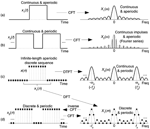
若函数在时(频)域是连续的,则其像函数在频(时)域是非周期的; 若函数在时(频)域是离散的,则其像函数在频(时)域是周期的。
| 傅立叶变换类型 | 时域 连续性 |
时域 周期性 |
频域 连续性 |
频域 周期性 |
|---|---|---|---|---|
| 连续傅立叶变换 Fourier Transform |
连续 | 非周期 | 连续 | 非周期 |
| 傅立叶级数 Fourier Series |
连续 | 周期 | 离散 | 非周期 |
| 离散时间傅立叶变换 Discrete-Time Fourier Transform (DTFT) |
离散 | 非周期 | 连续 | 周期 |
| 离散傅立叶变换 Discrete Fourier Transform (DFT) |
离散 | 周期 | 离散 | 周期 |
分别参见如下章节:
- 连续傅里叶变换 / Fourier Transform
- 傅里叶级数 / Fourier Series
- 离散时间傅里叶变换 / Discrete-Time Fourier Transform (DTFT)
- 离散傅里叶变换 / Discrete Fourier Transform (DFT)
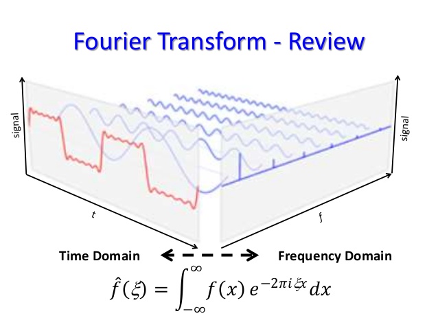
Fourier Transform
The Fourier transform decomposes a function of time (a signal) into the frequencies that make it up. The Fourier transform of a function of time itself is a complex-valued function of frequency, whose absolute value represents the amount of that frequency present in the original function, and whose complex value is the phase offset of the basic sinusoid in that frequency. The Fourier transform is called the frequency domain representation of the original signal.
The Fourier transform is not limited to functions of time, but in order to have a unified language, the domain of the original function is commonly referred to as the time domain. For many functions of practical interest one can define an operation that reverses this: the inverse Fourier transformation, also called Fourier synthesis, of a frequency domain representation combines the contributions of all the different frequencies to recover the original function of time.
Linear operations performed in one domain (time or frequency) have corresponding operations in the other domain, which are sometimes easier to perform. The operation of differentiation in the time domain corresponds to multiplication by the frequency, so some differential equations are easier to analyze in the frequency domain. Also, convolution in the time domain corresponds to ordinary multiplication in the frequency domain. Concretely, this means that any linear time-invariant system, such as a filter applied to a signal, can be expressed relatively simply as an operation on frequencies. After performing the desired operations, transformation of the result can be made back to the time domain. Harmonic analysis is the systematic study of the relationship between the frequency and time domains, including the kinds of functions or operations that are simpler in one or the other, and has deep connections to almost all areas of modern mathematics.
Definition
For an integrable function \(f(x)\),
| Fourier Transform | \(\hat{f}(\xi) = \int^{\infty}_{-\infty}f(x)e^{-2\pi ix\xi}dx\) |
| Inverse Fourier Transform | \(f(x) = \int^{\infty}_{-\infty}\hat{f}(\xi)e^{2\pi i\xi x}d\xi\) |
where,
- the independent variable x represents time (in seconds)
- the transform variable \(\xi\) represents frequency (in hertz)
- the functions f and \(\hat{f}\) often are referred to as a Fourier integral pair or Fourier transform pair
Properties of Fourier Transform
Refer to Fourier Transform Wikipedia (English) and Fourier Transform Wikipedia (Chinese).
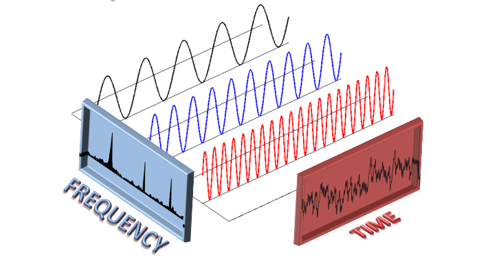
Fourier Transform Diagram
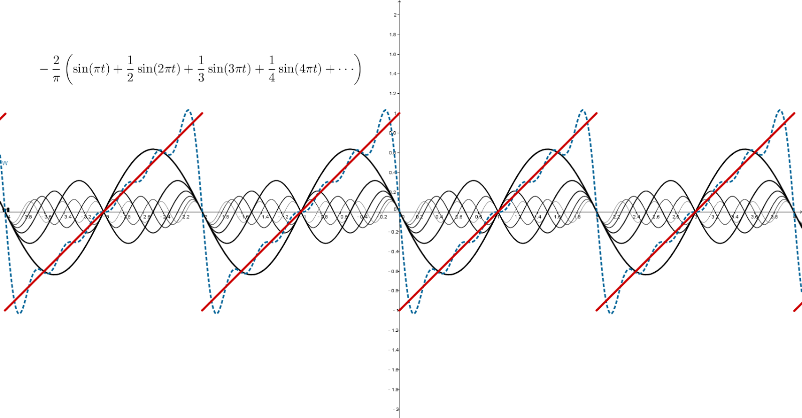
Fourier Series
The Fourier series decomposes any periodic function or periodic signal into the sum of a (possibly infinite) set of simple oscillating functions, namely sines and cosines (or, equivalently, complex exponentials). Fourier series are also central to the original proof of the Nyquist-CShannon sampling theorem. The study of Fourier series is a branch of Fourier analysis.
Definition
For periodic function \(f(t)\) with periodic T,
| Fourier Series | \(F_n = \frac{1}{T}\int^{T/2}_{-T/2}f(t)e^{-i2\pi nt/T}dt\) |
| Inverse Fourier Series | \(f(t) = \sum^{\infty}_{n=-\infty}F_ne^{i2\pi nt/T}\) |
| Inverse Fourier Series | If the periodic function \(f(t)\) is a real-valued function, then: \(f(t) = \frac{a_0}{2} + \sum^{\infty}_{n=1} {a_n cos(\frac{2\pi nt}{T}) + b_n sin(\frac{2\pi nt}{T})}\) |
Properties of Fourier Series
Refer to Fourier Series Wikipedia.
Fourier Series Diagram
方波 / Square Wave
锯齿波 / Sawtooth Wave
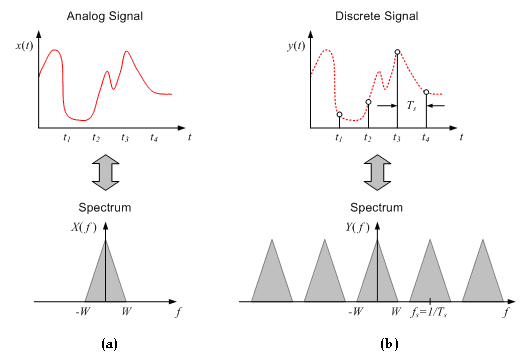
Nyquist-CShannon Sampling Theorem
在数字信号处理领域,奈奎斯特-香农采样定理是连续信号(通常称作”模拟信号”)与离散信号(通常称作”数字信号”)之间的一个基本桥梁。它确定了信号带宽的上限,或能捕获连续信号的所有信息的离散采样信号所允许的采样频率的下限。如果连续信号是带限的,并且采样频率大于信号带宽的2倍,那么原来的连续信号可以从采样样本中完全重建出来。
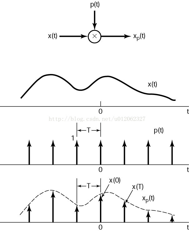
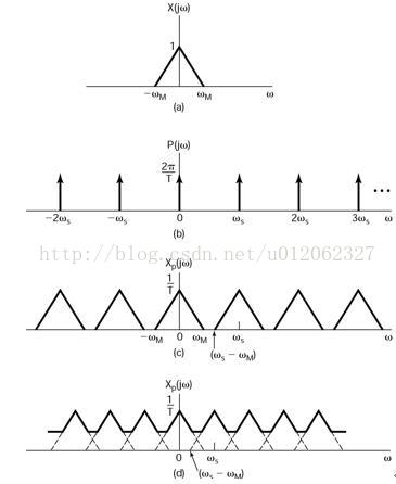
Discrete-Time Fourier Transform (DTFT)
In mathematics, the Discrete-Time Fourier Transform (DTFT) is a form of Fourier analysis that is applicable to the uniformly-spaced samples of a continuous function. The term discrete-time refers to the fact that the transform operates on discrete data (samples) whose interval often has units of time. From only the samples, it produces a function of frequency that is a periodic summation of the continuous Fourier transform of the original continuous function. Under certain theoretical conditions, described by the sampling theorem, the original continuous function can be recovered perfectly from the DTFT and thus from the original discrete samples. The DTFT itself is a continuous function of frequency, but discrete samples of it can be readily calculated via the discrete Fourier transform (DFT) (see Sampling the DTFT), which is by far the most common method of modern Fourier analysis.
Definition
Discrete-Time-Fourier-Transform-DTFT
DTFT Diagram
Discrete Fourier Transform (DFT)
The Discrete Fourier Transform (DFT) converts a finite sequence of equally spaced samples of a function into the list of coefficients of a finite combination of complex sinusoids, ordered by their frequencies, that has those same sample values. It can be said to convert the sampled function from its original domain (often time or position along a line) to the frequency domain.
Definition
For the sequence of N complex numbers \(x_0, x_1, \ldots, x_{N-1}\):
| Discrete Fourier Transform | \(X_k = \sum_{n=0}^{N-1}x_n e^{-2 \pi ikn/N}\) |
| Inverse Discrete Fourier Transform | \(x_n = \frac{1}{N} \sum_{n=0}^{N-1}X_k e^{2 \pi ikn/N}\) |
Using Euler’s formula, the DFT formulae can be converted to the trigonometric forms sometimes used in engineering and computer science.
| Discrete Fourier Transform | \(X_k = \sum_{n=0}^{N-1}x_n [cos(-2 \pi k \frac{n}{N}) + i \bullet sin(-2 \pi k \frac{n}{N})]\) |
| Inverse Discrete Fourier Transform | \(x_n = \frac{1}{N} \sum_{n=0}^{N-1}X_k [cos(2 \pi k \frac{n}{N}) + i \bullet sin(2 \pi k \frac{n}{N})]\) |
DFT Diagram
FFT and IFFT
A Fast Fourier transform (FFT) algorithm computes the Discrete Fourier transform (DFT) of a sequence, or its inverse. Fourier analysis converts a signal from its original domain (often time or space) to a representation in the frequency domain and vice versa. An FFT rapidly computes such transformations by factorizing the DFT matrix into a product of sparse (mostly zero) factors. As a result, it manages to reduce the complexity of computing the DFT from \(O(n^2)\), which arises if one simply applies the definition of DFT, to \(O(n \bullet logn)\), where n is the data size.
Algorithms
- Cooley-CTukey FFT algorithm
- Prime-factor FFT algorithm
- Bruun’s FFT algorithm
- Rader’s FFT algorithm
- Bluestein’s FFT algorithm
- …
References
- Fourier Transform Wikipedia (English)
- Fourier Transform Wikipedia (Chinese)
- 傅立叶变换家族中的关系
- Fourier Series Wikipedia
- 奈奎斯特-香农采样定理
- Discrete Fourier transform (DFT) Wikipedia
- Discrete-Time Fourier Transform (DTFT) Wikipedia
- Fast Fourier Transform (FFT) Wikipedia
- 不看任何数学公式来讲解傅里叶变换 local pdf
- 傅里叶变换:MP3、JPEG和Siri背后的数学 local pdf
- MATLAB
- SciLab