Digital Pre-Distortion (DPD)
This article introduce the Digital Pre-Distortion (DPD).
Taylor Expansion / 泰勒展开式
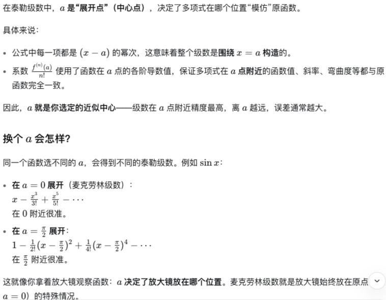
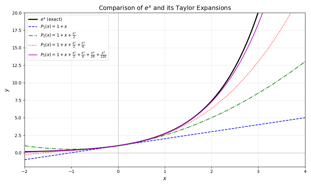
Exponential function and its Taylor expansion
import numpy as np
import matplotlib.pyplot as plt
import math

def taylor_exp(x, n):
    result = 0
    for k in range(n+1):
        result += x**k / math.factorial(k)
    return result

x = np.linspace(-2, 4, 300)
y_exp = np.exp(x)

y_t1 = taylor_exp(x, 1)
y_t2 = taylor_exp(x, 2)
y_t3 = taylor_exp(x, 3)
y_t5 = taylor_exp(x, 5)

plt.figure(figsize=(10, 6))
plt.plot(x, y_exp, 'k-', linewidth=2.5, label=r'$e^x$ (exact)')
plt.plot(x, y_t1, 'b--', label=r'$P_1(x)=1+x$')
plt.plot(x, y_t2, 'g-.', label=r'$P_2(x)=1+x+\frac{x^2}{2}$')
plt.plot(x, y_t3, 'r:', label=r'$P_3(x)=1+x+\frac{x^2}{2}+\frac{x^3}{6}$')
plt.plot(x, y_t5, 'm-', linewidth=1.5, label=r'$P_5(x)=1+x+\frac{x^2}{2}+\frac{x^3}{6}+\frac{x^4}{24}+\frac{x^5}{120}$')

plt.axhline(0, color='gray', linewidth=0.5)
plt.axvline(0, color='gray', linewidth=0.5)
plt.xlim(-2, 4)
plt.ylim(-2, 20)
plt.grid(alpha=0.3)

plt.title(r'Comparison of $e^x$ and its Taylor Expansions', fontsize=14)
plt.xlabel(r'$x$', fontsize=12)
plt.ylabel(r'$y$', fontsize=12)
plt.legend(loc='upper left', fontsize=10)
plt.tight_layout()
plt.show()
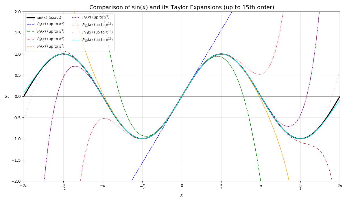
Sinx function and its Taylor expansion
import numpy as np
import matplotlib.pyplot as plt
import math

def sin_taylor(x, max_power):
    """
    计算 sin(x) 的泰勒多项式,保留所有奇次项直到指定最高幂次 max_power (奇数)
    例如 max_power=15 将包含 x, x^3, x^5, ..., x^15
    """
    result = 0
    k = 0
    while 2*k + 1 <= max_power:
        coef = (-1)**k / math.factorial(2*k + 1)
        result += coef * (x ** (2*k + 1))
        k += 1
    return result

# x 轴范围:-2π 到 2π
x = np.linspace(-2*np.pi, 2*np.pi, 800)

# 精确 sin(x)
y_sin = np.sin(x)

# 定义要展示的阶数(最高幂次)
powers = [1, 3, 5, 7, 9, 11, 13, 15]
colors = ['blue', 'green', 'red', 'orange', 'purple', 'brown', 'pink', 'cyan']
linestyles = ['--', '-.', ':', (0, (5, 1)), (0, (3, 1, 1, 1)), (0, (5, 5)), (0, (3, 5, 1, 5)), '-']

plt.figure(figsize=(12, 7))
plt.plot(x, y_sin, 'k-', linewidth=2.5, label=r'$\sin(x)$ (exact)')

for power, color, ls in zip(powers, colors, linestyles):
    y_approx = sin_taylor(x, power)
    plt.plot(x, y_approx, color=color, linestyle=ls, linewidth=1.2,
             label=rf'$P_}(x)$ (up to $x^}$)')

# 辅助线
plt.axhline(0, color='gray', linewidth=0.5)
plt.axvline(0, color='gray', linewidth=0.5)
plt.xlim(-2*np.pi, 2*np.pi)
plt.ylim(-2, 2)

# 设置 x 轴刻度为 π 的倍数
xticks = [-2*np.pi, -3*np.pi/2, -np.pi, -np.pi/2, 0, np.pi/2, np.pi, 3*np.pi/2, 2*np.pi]
xtick_labels = [r'$-2\pi$', r'$-\frac{3\pi}{2}$', r'$-\pi$', r'$-\frac{\pi}{2}$',
                '0', r'$\frac{\pi}{2}$', r'$\pi$', r'$\frac{3\pi}{2}$', r'$2\pi$']
plt.xticks(xticks, xtick_labels)

plt.grid(alpha=0.3)
plt.title(r'Comparison of $\sin(x)$ and its Taylor Expansions (up to 15th order)', fontsize=14)
plt.xlabel(r'$x$', fontsize=12)
plt.ylabel(r'$y$', fontsize=12)
plt.legend(loc='upper left', fontsize=9, ncol=2)  # 分成两列,避免图例过长
plt.tight_layout()
plt.show()
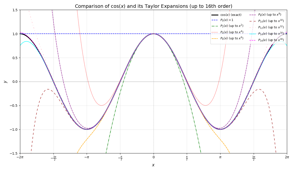
Cosx function and its Taylor expansion
import numpy as np
import matplotlib.pyplot as plt
import math

def cos_taylor(x, max_power):
    """
    计算 cos(x) 的泰勒多项式,保留所有偶次项直到指定最高幂次 max_power (偶数)
    例如 max_power=16 将包含 1, x^2, x^4, ..., x^16
    """
    result = 0
    k = 0
    while 2*k <= max_power:
        coef = (-1)**k / math.factorial(2*k)
        result += coef * (x ** (2*k))
        k += 1
    return result

# x 范围:-2π 到 2π
x = np.linspace(-2*np.pi, 2*np.pi, 800)

# 精确 cos(x)
y_cos = np.cos(x)

# 要显示的阶数(最高幂次)
powers = [0, 2, 4, 6, 8, 10, 12, 14, 16]
colors = ['blue', 'green', 'red', 'orange', 'purple', 'brown', 'pink', 'cyan', 'magenta']
linestyles = ['--', '-.', ':', (0, (5, 1)), (0, (3, 1, 1, 1)), (0, (5, 5)), (0, (3, 5, 1, 5)), '-', '--']

plt.figure(figsize=(12, 7))
plt.plot(x, y_cos, 'k-', linewidth=2.5, label=r'$\cos(x)$ (exact)')

for power, color, ls in zip(powers, colors, linestyles):
    if power == 0:
        label = r'$P_0(x)=1$'
    else:
        label = rf'$P_}(x)$ (up to $x^}$)'
    y_approx = cos_taylor(x, power)
    plt.plot(x, y_approx, color=color, linestyle=ls, linewidth=1.2, label=label)

# 辅助线
plt.axhline(0, color='gray', linewidth=0.5)
plt.axvline(0, color='gray', linestyle=':', linewidth=0.5)
plt.xlim(-2*np.pi, 2*np.pi)
plt.ylim(-1.5, 1.5)

# x 轴刻度为 π 的倍数
xticks = [-2*np.pi, -3*np.pi/2, -np.pi, -np.pi/2, 0, np.pi/2, np.pi, 3*np.pi/2, 2*np.pi]
xtick_labels = [r'$-2\pi$', r'$-\frac{3\pi}{2}$', r'$-\pi$', r'$-\frac{\pi}{2}$',
                '0', r'$\frac{\pi}{2}$', r'$\pi$', r'$\frac{3\pi}{2}$', r'$2\pi$']
plt.xticks(xticks, xtick_labels)

plt.grid(alpha=0.3)
plt.title(r'Comparison of $\cos(x)$ and its Taylor Expansions (up to 16th order)', fontsize=14)
plt.xlabel(r'$x$', fontsize=12)
plt.ylabel(r'$y$', fontsize=12)
plt.legend(loc='upper right', fontsize=9, ncol=2)
plt.tight_layout()
plt.show()
Volterra series / 沃尔泰拉级数
Volterra级数由意大利数学家Vito Volterra在20世纪初引入。Volterra的研究主要集中在积分方程和函数分析方面,他在非线性系统理论中做出了重要贡献。Volterra级数的提出,为解决复杂非线性系统提供了一种新的方法。
Volterra级数是一种描述非线性动态系统(带记忆的非线性系统)输入-输出关系的泛函级数。如果把泰勒级数看作”无记忆非线性”的展开,Volterra级数就是带记忆的泰勒级数,能够刻画系统不仅依赖于当前输入,还依赖于过去的输入。
Memory Polynomial (MP) / 记忆多项式
import numpy as np
import matplotlib.pyplot as plt

# 扩展记忆多项式模型(M=5, K=7 奇数阶)
def memory_polynomial_extended(x, coeff_dict):
    M = 5  # 记忆深度
    y = np.zeros_like(x, dtype=complex)
    for n in range(len(x)):
        total = 0.0 + 0.0j
        for m in range(M+1):
            if n - m >= 0:
                xm = x[n-m]
                for p in [1,3,5,7]:
                    a = coeff_dict.get((m, p), 0.0)
                    total += a * xm * (np.abs(xm) ** (p-1))
        y[n] = total
    return y

# ---------- 系数设置(与之前相同) ----------
coeff = {}
np.random.seed(42)
for m in range(6):   # m=0..5
    decay = np.exp(-m / 2.0)
    coeff[(m,1)] = (0.9 * decay) * np.exp(1j * 0.05 * m)
    coeff[(m,3)] = (-0.08 * decay) * np.exp(1j * 0.2)
    coeff[(m,5)] = (0.02 * decay) * np.exp(1j * 0.3)
    coeff[(m,7)] = (-0.005 * decay) * np.exp(1j * 0.1)

# ---------- 1. 扫幅输入:AM-AM 和 AM-PM ----------
A = np.linspace(0, 1.8, 300)
x_sweep = A + 0j
y_sweep = memory_polynomial_extended(x_sweep, coeff)

out_amp = np.abs(y_sweep)
out_phase_deg = np.angle(y_sweep, deg=True)

# ---------- 2. 矩形脉冲输入:记忆效应 ----------
t = np.arange(0, 80)
x_pulse = np.zeros_like(t, dtype=complex)
x_pulse[20:35] = 1.0
y_pulse = memory_polynomial_extended(x_pulse, coeff)

# ---------- 绘图:两行布局 ----------
plt.figure(figsize=(12, 8))   # 宽度较大,高度适中

# 第一行,第一列:AM-AM
plt.subplot(2, 2, 1)
plt.plot(A, out_amp, 'b-', linewidth=2, label='Memory poly (M=5,K=7)')
plt.plot(A, A, 'r--', alpha=0.6, label='Ideal')
plt.xlabel('Input amplitude')
plt.ylabel('Output amplitude')
plt.title('AM‑AM characteristic')
plt.grid(True)
plt.legend()

# 第一行,第二列:AM-PM
plt.subplot(2, 2, 2)
plt.plot(A, out_phase_deg, 'g-', linewidth=2)
plt.xlabel('Input amplitude')
plt.ylabel('Phase shift (degrees)')
plt.title('AM‑PM characteristic')
plt.grid(True)

# 第二行,合并两列:脉冲响应
plt.subplot(2, 2, (3, 4))   # 或者使用 subplot(2,1,2) 但保持 2x2 结构更方便
plt.plot(t, np.abs(x_pulse), 'r-', label='Input amplitude')
plt.plot(t, np.abs(y_pulse), 'b-', label='Output amplitude (M=5)')
plt.xlabel('Sample index')
plt.ylabel('Amplitude')
plt.title('Memory effect: response to a rectangular pulse')
plt.grid(True)
plt.legend()

plt.tight_layout()
plt.show()
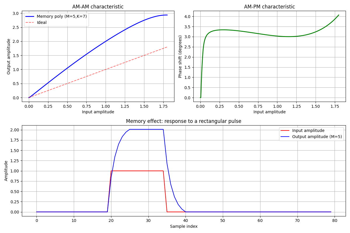
运行结果说明:
- AM‑AM 图(第1行):输出幅度随输入幅度的变化。由于三次、五次等负系数项的贡献,呈现饱和压缩特性(蓝色曲线低于红色理想直线)。
- AM‑PM 图(第2行):输出相位随输入幅度的变化。由于系数为复数,输入为实信号时输出产生相位偏移,体现了非线性相位失真。
- 脉冲响应图(第3行):输入为矩形脉冲(红色),输出幅度(蓝色)在脉冲结束后仍有明显的”拖尾”,且拖尾长度与记忆深度 M=5 相关,清晰展示了记忆效应。
参数调整说明:
- 您可以根据实际需要修改 coeff 字典中的系数值(幅度和相位),以模拟不同的非线性特性。
- 记忆深度 M 和非线性阶数 K 已按您的要求设定为最大 5 和 7,如需扩展,可修改函数中的
range(M+1)和[1,3,5,7]列表。
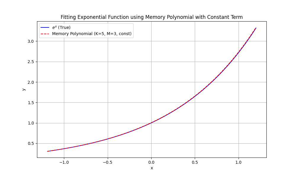
用记忆多项式拟合指数函数
import numpy as np
import matplotlib.pyplot as plt

class MemoryPolynomial:
    """
    Memory polynomial model with optional constant term.
    y(n) = c + Σ_{m=0}^{M-1} Σ_{k=0}^{K-1} a_{m,k} * x(n-m) * |x(n-m)|^k
    """
    def __init__(self, K, M, use_abs=False, include_const=False):
        self.K = K                # polynomial order (number of basis functions per memory tap)
        self.M = M                # memory depth
        self.use_abs = use_abs    # whether to use |x|^k  (default: x^k)
        self.include_const = include_const
        self.coeffs = None        # coefficients: shape (M, K) if no const, else (M, K) + const scalar
        self.const = None

    def _build_design_matrix(self, x):
        N = len(x)
        L = N - self.M + 1        # number of valid output samples
        n_basis = self.M * self.K
        if self.include_const:
            n_basis += 1
        X = np.zeros((L, n_basis))
        for n in range(self.M-1, N):
            row_idx = n - self.M + 1
            col = 0
            # memory terms
            for m in range(self.M):
                xnm = x[n - m]
                if self.use_abs:
                    base = abs(xnm)
                else:
                    base = xnm
                for k in range(self.K):
                    X[row_idx, col] = xnm * (base ** k)
                    col += 1
            # constant term
            if self.include_const:
                X[row_idx, col] = 1.0
        return X

    def fit(self, x, y):
        assert len(x) == len(y), "x and y must have same length"
        N = len(x)
        L = N - self.M + 1
        if L <= 0:
            raise ValueError(f"Sequence length must be greater than memory depth M={self.M}")
        X = self._build_design_matrix(x)
        y_trim = y[self.M-1:]    # align with valid rows
        # least squares
        coeffs_full = np.linalg.lstsq(X, y_trim, rcond=None)[0]
        # split coefficients
        n_mem_basis = self.M * self.K
        if self.include_const:
            self.coeffs = coeffs_full[:n_mem_basis].reshape(self.M, self.K)
            self.const = coeffs_full[-1]
        else:
            self.coeffs = coeffs_full.reshape(self.M, self.K)
            self.const = 0.0

    def predict(self, x):
        N = len(x)
        y_pred = np.zeros(N)
        for n in range(self.M-1, N):
            val = self.const   # constant term
            for m in range(self.M):
                xnm = x[n - m]
                if self.use_abs:
                    base = abs(xnm)
                else:
                    base = xnm
                for k in range(self.K):
                    val += self.coeffs[m, k] * xnm * (base ** k)
            y_pred[n] = val
        # first M-1 points cannot be computed due to missing history
        y_pred[:self.M-1] = np.nan
        return y_pred


# ---------------------- Parameters ----------------------
K = 5          # polynomial order (x^1 ... x^K)
M = 3          # memory depth
use_abs = False
include_const = True   # add constant term

# Generate training data on [-1, 1]
x_train = np.linspace(-1, 1, 200)
y_train = np.exp(x_train)

# Create and fit model
mp = MemoryPolynomial(K, M, use_abs, include_const)
mp.fit(x_train, y_train)

# Test data on a slightly larger interval
x_test = np.linspace(-1.2, 1.2, 500)
y_true = np.exp(x_test)
y_pred = mp.predict(x_test)   # first M-1 entries are NaN

# Remove NaN for plotting and error calculation
valid_idx = ~np.isnan(y_pred)
x_test_valid = x_test[valid_idx]
y_true_valid = y_true[valid_idx]
y_pred_valid = y_pred[valid_idx]

# ---------------------- Plot ----------------------
plt.figure(figsize=(10, 6))
plt.plot(x_test_valid, y_true_valid, 'b-', label=r'$e^x$ (True)')
plt.plot(x_test_valid, y_pred_valid, 'r--', label=f'Memory Polynomial (K={K}, M={M}, const)')
plt.title('Fitting Exponential Function using Memory Polynomial with Constant Term')
plt.xlabel('x')
plt.ylabel('y')
plt.legend()
plt.grid(True)
plt.show()

# Errors
mse = np.mean((y_pred_valid - y_true_valid)**2)
max_err = np.max(np.abs(y_pred_valid - y_true_valid))
print(f"Test MSE: {mse:.2e}")
print(f"Test Maximum Absolute Error: {max_err:.2e}")

# Display coefficients
print("\nConstant term: {:.6f}".format(mp.const))
print("Memory polynomial coefficients (a_{m,k}) for m=0..M-1, k=0..K-1 (basis: x * |x|^k):")
for m in range(M):
    for k in range(K):
        print(f"  m={m}, k={k}: {mp.coeffs[m, k]:.6f}")
Why Memory Polynomial (MP) can be used in DPD?
Generalized Memory Polynomial (GMP) / 广义记忆多项式
- Digital Pre-Distortion for RF Communications: From quations to Implementation, Chinese
- Digital Pre-Distortion for RF Communications: From quations to Implementation, English
DPD Overview
- DPD Basic Introduction
- Digital Pre-Distortion (DPD)
- Digital Pre-Distortion (DPD) Concept
- Theory of Operation for Digital Predistortion
- Linearization DesignGuide Reference
- Practical Digital Pre-Distortion (DPD) Techniques for PA Linearization in 3GPP LTE
- Ultrawideband Digital Pre-Distortion (DPD): The Rewards (Power and Performance) and Challenges of Implementation in Cable Distribution Systems: online, pdf
- A Polynomial Digital Pre-Distortion Technique Based on Iterative Architecture: pdf
- Digital Pre-Distortion Using Machine Learning Algorithms: pdf
- 功放数字预失真线性化技术发展趋势与挑战: pdf
- 何为CFR & DPD